Simple Software Verification, Part 3: Karnaugh Maps
(Image by Ben Laposky)
[hamzh_toggle title=”Series Parts” state=”closed”]
- Part 1 – Execution Tables
- Part 2 – Trace Tables
- Part 3 – Karnaugh Maps
[/hamzh_toggle]
Welcome to the third and final article in this mini-series on software validation. In this article we’re going to discuss state machines, what desirable properties they should possess, and then I’ll demonstrate a simple tool for verifying them called Karnaugh Maps.
Identifying State Machines
As a general rule of thumb, you can identify a program that is a potential candidate for state machine implementation by asking a simple question: “Can the program behave differently with identical inputs?” In other words, does your program use extra information (state) to determine how an input is processed. If so, you probably have a state machine, and depending on the number of states, it may be useful to formalize this.
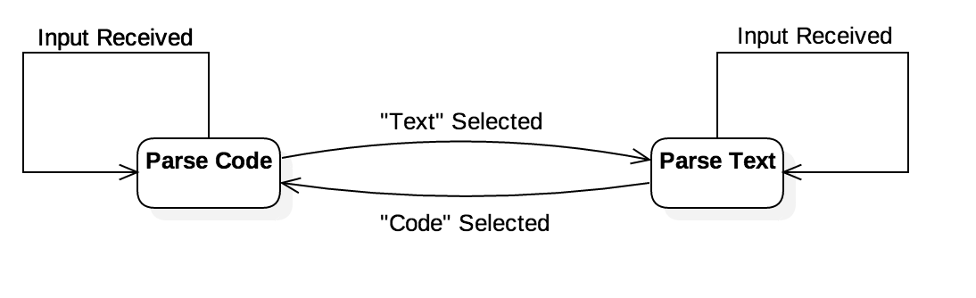
As an example of such a program, imagine we had an application that parsed user input as code if the “Code” tab was selected or parsed it as “Text” if another tab was selected. This program clearly behaves differently given identical user inputs. Specifically, it depends on which tab we’re typing in. So, it passes our simple state machine test. Its visual state machine representation would be something like the following:
Desirable Properties for Verification
Once you have identified an element as a state-machine and thoroughly defined it as such, another question arises. How do I know that my state machine will work? To answer this question, it would be nice to have some sort of criteria for what “will work” means. With state machines this criteria is simple to define. We are looking for two key properties:
- Completeness – All states are accounted for. No inputs produce an undefined state.
- Orthogonality – State transition conditions do not overlap.
While we could manually inspect the state machine and hope to correctly identify these properties, there’s an easier way: Karnaugh Maps
Karnaugh Maps
Karnaugh Maps are a visual aid for verifying state machines. In constructing a Karnaugh Map you will build a table showing all possible combinations of the available state variables. You can then inspect this table to easily identify Completeness and Orthogonality. In a Karnaugh Map, we can identify our desirable state machine properties by the following:
- Completeness – All cells of the table have an entry.
- Orthogonality – All cells have one, and only one, entry.
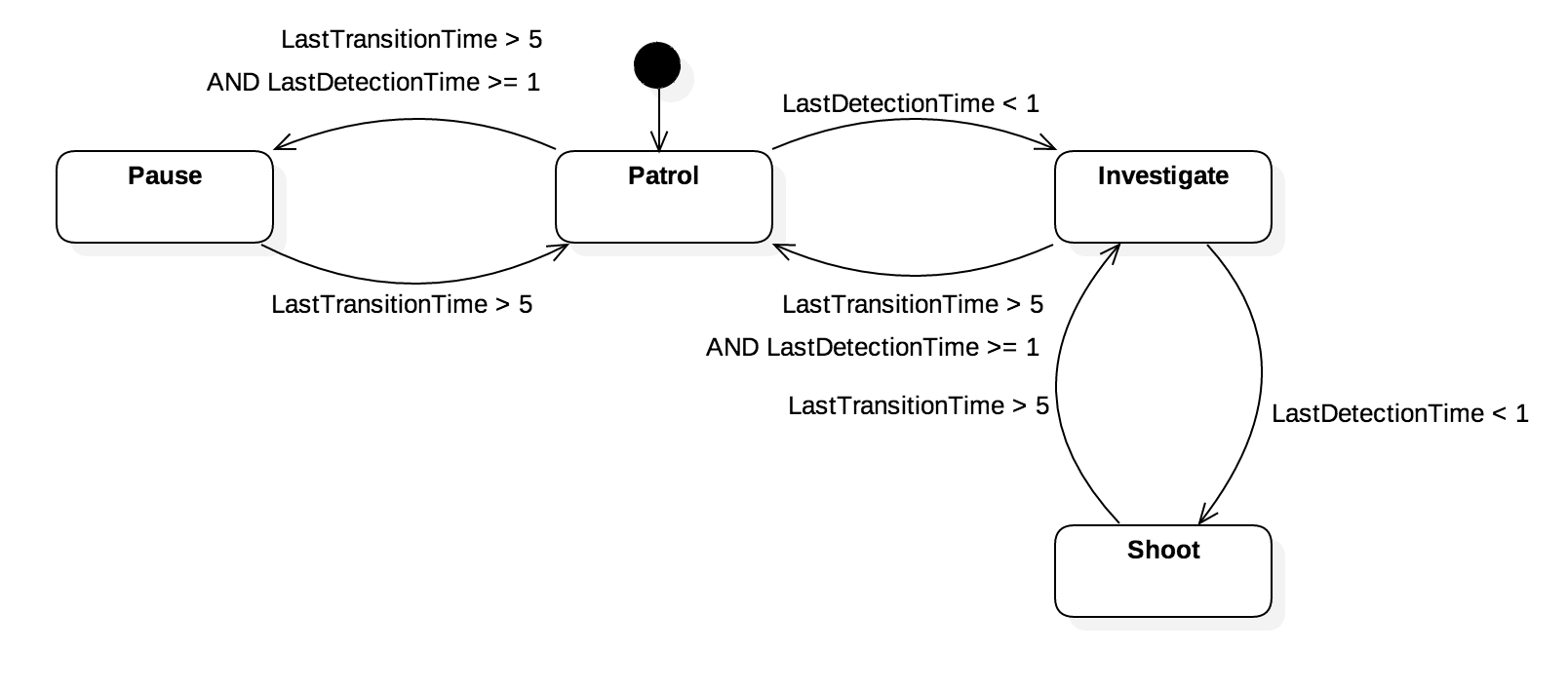
To demonstrate how Karnaugh maps can help you see potential issues with your state machines, let’s look at a simple example, a sentry in a video game. When not investigating or shooting, our sentry will patrol the grounds, pausing occasionally to ponder life and look around. This looks something like the following:

The sentry state machine has two variables. LastTransitionTime represents the time ago, in seconds, that we last transitioned states. LastDetectionTime represents the time ago, in seconds, that we last detected something. We can now construct a Karnaugh Map to tell us if our state transitions are Complete and Orthogonal. We’ll abbreviate the states as P (Patrol), PS (Pause), I (Investigate), and S (Shoot).
| LastTransitionTime <= 5 | LastTransitionTime > 5 | |||
| LastDetectionTime < 1 | LastDetectionTime >= 1 | LastDetectionTime < 1 | LastDetectionTime >= 1 | |
| P | I | P | PS, I | PS |
| PS | PS | PS | P | P |
| I | S | I | P, S | P |
| S | S | S | I | I |
Immediately we can see that this state machine is Complete, but it IS NOT Orthogonal. Namely, when LastTransitionTime > 5 and LastDetectionTime < 1. We can see this because there are two cells in this column with more than one entry. This represents a conflict where two different state transitions are equally valid. There are some state machines where this may be desirable, for example with Non-Deterministic Finite Automata, but for our purposes here this won’t work.
This non-orthogonality tells us that we need to better specify these state transitions. We can now revise the state machine so that one and only one of the two conflicting state transitions is allowed. For example, here is one possible revision:
This fix works because we now decide a precedence between LastDetectionTime and LastTransitionTime. Here we give precedence to LastDetectionTime. The Karnaugh Map for this revised state machine now looks like:
| LastTransitionTime <= 5 | LastTransitionTime > 5 | |||
| LastDetectionTime < 1 | LastDetectionTime >= 1 | LastDetectionTime < 1 | LastDetectionTime >= 1 | |
| P | I | PS | PS | PS |
| PS | PS | PS | P | P |
| I | S | I | P | P |
| S | S | S | I | I |
Now we can see that we have both a Complete and an Orthogonal state machine. Easy-peasy.
Conclusion
As you can see, Karnaugh Maps are a great tool for debugging state machine behavior. They are also pretty quick to construct, so if you ever find yourself building a state machine, it’s not very time-consuming to construct a Karnaugh Map to prove its Complete and Orthogonal while you’re at it.
That being said, the observant reader may have noticed that as the number of state variables increases, Karnaugh Maps seem to get quickly out of hand. In cases where your state machines become extremely complex it may begin to make sense to use a formal specification language language like TLA+ or Alloy. These tools can help you define and test your state machines to ensure there are no undefined transitions.
If you’ve been following along in this series, thank you. We’ve only scratched the surface of formal verification techniques, but my hope is that they’ve been made less intimidating and more accessible. If you want to dive deeper, see the additional reading section below for some great places to start.
Additional Reading
- A Discipline for Software Engineering – Book. Covers other software verification techniques.
- Specifying Systems – Free Ebook. Leslie Lamport on specifying systems in TLA+.
- TLA Homepage – Website. Microsoft research page on TLA+.
- Thinking Above Code – Video. Talk by Leslie Lamport on need for formal specification and other tools for thinking about our programs.
- Thinking For Programmers – Video. Another talk by Leslie Lamport.
Related Posts